Ed. Note: this post is again in my voice, but co-written with Kevin Jamieson. Kevin provided all of the awesome plots, and has a great tutorial for implementing the algorithm I’ll describe in this post

In the last post, I argued that random search is a competitive method for black-box parameter tuning in machine learning. This is actually great news! Random search is a incredibly simple algorithm, and if it is as powerful as anything else we’ve come up with so far, we can devote our time to optimizing random search for the particularities of our workloads, rather than worrying about baking off hundreds of new algorithmic ideas.

In some very nice recent work, Kevin Jamieson and Ameet Talwalkar pursued a very nice direction in accelerating random search. Their key insight is that most of the algorithms we run are iterative in machine learning, so if we are running a set of parameters, and the progress looks terrible, it might be a good idea to quit and just try a new set of hyperparameters.

One way to implement such a scheme called successive halving. The idea successive halving is remarkably simple. We first try out $N$ hyperparameter settings for some fixed amount of time $T$. Then, we keep the $N/2$ best performing algorithms and run for time $2T$. Repeating this procedure $\log_2(M)$ times, we end up with $N/M$ configurations run for $MT$ time.

The total amount of computation in each halving round is equal to $NT$, and there are $\log_2(M)$ total rounds. If we restricted ourself to pure random search with the same computation budget (i.e., $NT\log_2(M)$ time steps) and required each of the chosen parameter settings to be run for $MT$ steps, we would only be able to run $N \log_2(M)/M$ hyperparameter settings. Thus, in the same amount of time, successive halving sees $M/\log_2(M)$ more parameter configurations than pure random search!

Now, the problem here is that just because an parameter setting looks bad at the beginning of a run of SGD, doesn’t meant that it won’t be optimal at the end of the run. We see this a lot when tuning learning rates: slow learning rates are often poor for the first couple of epochs, but end up with the lowest test error after a hundred passes over the data.

A simple way to deal with this tradeoff between breadth and depth is to start the halving process later. We could run $N/2$ parameter settings for time $2T$, then the top $N/4$ for time $4T$ and so on. This adapted halving scheme allows slow learners to have more of a chance of surviving before being cut, but the total amount of time per halving round is still $N$ and the number of rounds is at most $\log_2(M)$. Running multiple instances of successive halving with different halving times increases depth while narrowing depth.

Following up on Kevin and Ameet’s initial work, Lisha Li, Kevin Jamieson, Giulia DeSalvo, Afshin Rostamizadeh, and Ameet Talwalkar recently provided a simple, automatic way to balance these breadth-versus-depth tradeoffs. The algorithm is remarkably simple: see Kevin’s project page for the 7 lines of python code. The only parameters you need to know to generate a search protocol is the minimum amount of time you’d like to run your model before checking against other models and the maximum amount of time you’d ever be interested in running for. In the examples above, the minimum time was $T$ and the maximum time was $MT$. In some sense, these parameters are more like constraints: there is some overhead with checking the process, and the minimum time should be larger than this. The maximum runtime is here because we all have deadlines. The only parameter that needs to be given to Kevin’s code is $M$ (which he calls max_iter).

Successive halving was inspired by an earlier heuristic by Evan Sparks and coauthors which showed the simple idea of killing iterative jobs based on early progress worked really well in practice. The version described above is an adaptation of the algorithm proposed by Karnin, Koren, and Somekh for stochastic Multi-armed bandits. Li et al provide a multiround scheme (which they call Hyperband) that adapts the scheme of Karnin et al to finite horizon, non-stochastic search. Li et al describe a number of extensions of the scheme for other machine learning workloads, many interesting theoretical guarantees, and implications for stochastic infinite-armed bandit problems (if you’re into that sort of thing). Let’s wrap up this blogpost with some empirical evidence that this algorithm actually works.

Neural net experiments

Let’s look at three small image classification benchmarks: CIFAR-10, the Street View House Numbers (SVHN), and rotated MNIST with background images (MRBI). The CIFAR-10 and SVHN data sets contain 32 × 32 RGB images. MRBI contains 28 x 28 grayscale images. Each dataset is split into a training, validation, and test set: (1) CIFAR-10 has 40,000, 10,000, and 10,000 instances; (2) SVHN has close to 600,000, 6,000, and 26,000 instances. (3) MRBI has 10,000 , 2,000, and 50,000 instances for training, validation, and test respectively.

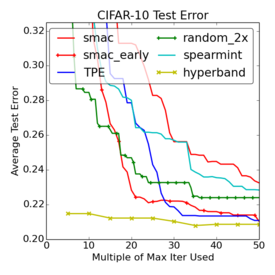
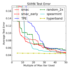
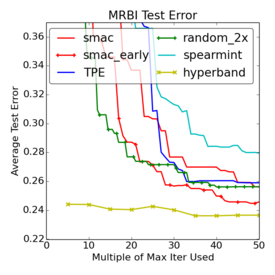
For the experts out there, the goal is to tune the basic cuda-convnet model, searching for the optimal learning rate, learning rate decay, $\ell_2$ regularization parameters on different layers, and parameters of the response normalizations. For both datasets, the basic unit of time, $T$, was 10,000 examples. For CIFAR-10 this was one-fourth of an epoch, and $M$ was 300, equivalent to 75 epochs over the 40,000 example training set. For SVHN, $T$ corresponded to one-sixtieth of an epoch and $M$ was set to 600, equivalent to 10 epochs over the 600,000 example training set. For MRBI, $T$ was one epoch and $M$ was 300. The full details of these experiments are described in the paper. The plots below compare the performance of the Hyperband algorithm to a variety of other hyperparameter tuning algorithms. In particular, as raised in the comments in the previous post, we are comparing to Spearmint, a very popular Bayesian optimization scheme and SMAC-early which is a variant of SMAC that is designed to incorporate early stopping. The following plots are curves of the mean of 10 trials (not the min of 10 trials).

First, note that Random-2x is again a very competitive algorithm. None of the pure Bayesian optimization methods outperform Random-2x on all three data sets. Only SMAC-early, with its ability to stop underperforming jobs, is able to consistently outperform Random-2x.

The comparison to Hyperband, on the other hand, is striking. On average, Hyperband finds a decent solution in a fraction of the time of all of the other methods. It also finds the best solution over all in all three cases. On SVHN, it finds the best solution in a fifth of the time of the other methods. And, again, the protocol is just 7 lines of python code. Hyperband is just a first step, and other might not be the ideal solution for your particular workload. But I think these plots nicely illustrate how simple-but enhancements of random search can go a very long way.